 |
PageBox |
| Support | Map |
|
|
|
|
|
|
|
|
Graph introduction
| Table of content | |
|
A graph is a pair G = (V, E) where V is a set of vertices and E is a binary relation on V.
E contains a pair (u, v) if there is an edge between the u and v vertices.
If the graph is directed, this pair is ordered: (u, v) is not the same as (v, u).
Directed graph: Edges go from one vertex to another in a specific direction
Undirected graph: Edges have no direction
Adjacency: If a graph contains the edge (u, v) then v is adjacent to u
Completeness: A graph in which every vertex is adjacent to each other is called complete
Incidence: In a directed graph an edge (u, v) is incident from u and is incident to v. The in-degree of a vertex is the number of edges incident to it. The out-degree of a vertex is the number of edges incident from it.
Path: A path is a sequence of vertices traversed by following the edges between them
Cycle: A cycle is a path that includes the same vertex two or more times. A graph without cycles is acyclic. Directed Acyclic Graphs are called dags.
Articulation: If removing a vertex disconnects a graph the vertex is an articulation point
Weighted graph: In a weighted graph, each edge is assigned a weight value
Hamiltonian-cycle: Path that passes through every vertex exactly once before returning to the original vertex. Superset of traveling salesman.
Clique: A clique is a region of a graph where each vertex is connected to the others. We present a clique application in our NWS presentation. In this case graph vertices are computers. A clique can be made of the computer connected to the same sub-network.
Examples:
Minimum spanning tree
Finding the shortest path
Solving the traveling-salesman problem. The salesman needs to meet customers in a number of cities (vertices) and wants to find the shortest path route (sum of edges) by which he can visit every city exactly once before returning to the point at which he starts.
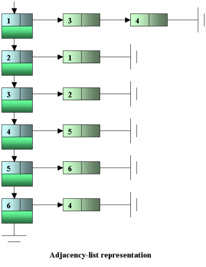
The most common way to represent a graph is an adjacency-list representation.
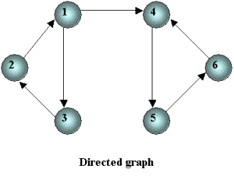
Given the graph below:

We can represent it with:

Another representation is a adjacency matrix. For a graph with V vertices, a V x V matrix is used where each element V[i, j] is a Boolean that says whether there is an edge from vertex i to vertex j.
The advantage of this matrix format over the adjacency list is that edge insertion and removal is constant time. It tends to use more memory than adjacency list. It is better to use the matrix for dense graphs where the number of edges is close to the number of elements in the matrix and to use an adjacency list when the graph is sparse.
Breadth-first search explores a graph by visiting all vertices adjacent to a vertex.
Then it repeats the process for each vertex discovered.
Breadth-first search is useful for instance to compute the shortest path between each pair of vertices.
Depth-first search explores a graph by first visiting undiscovered vertices adjacent to the most recently discovered vertex.
Depth-first search is useful for instance to detect cycles.
The goal of a graph partitioner, also called mesh partitioner, is to separate the vertices of a graph into almost equal-sized components such that the number of edges between components is minimized. Finding good graph partitions has been the focus of much recent research because it can be used to reduce the communication among processors in a parallel machine. In particular if the graph represents the communication structure of a set of entities, then the graph partitioner can be used to allocate the entities to processors such that communication is reduced.
Most graph partitioners work with undirected graphs. They often use geometric algorithms (they try to draw a line that cuts a minimum number of edges). Geometric algorithms also imply that we can provide the coordinates of the vertices.
You can look at http://www-2.cs.cmu.edu/~scandal/alg/separator.html for examples of graph partitioners. On this page three kinds of partitioners are described:
Coordinate bisection: This algorithm considers each axis (x, y or z in three dimension) and takes a median along that axis. It then measures the number of edges that will be cut if we separate the vertices into the ones less and greater than the median. It selects the axis (one of x, y or z) that minimizes the number of edges cut.
Random Circles: This technique due to Miller, Teng, Thurston and Vavasis, is also geometric in nature. Instead of making planar cuts as in the coordinate bisection, it makes spherical cuts (or circular in 2 dimensions). These cuts are made by projecting the vertices onto the surface of a sphere in one higher dimension and then making a planar cut on that sphere (these cuts will transform into spherical cuts when projected back into the lower dimension).
Spectral bisection: This algorithm is based on finding the second eigenvector of the Laplacian of the graph. A Laplacian matrix is a sort of adjacency matrix. It is possible to find vectors, called Eigenvectors that satisfy to the equation: Laplace_matrix * Eigenvector = Eigenvalue * Eigenvector where Eigenvalue is a number. The eigenvector is then sorted and all the vertices are split based on amplitude.
There are parallel graph partitioner that run in an MPI or PVM environment. See our Grid page for more information about MPI and PVM. You can check MIST for instance. You can also look at METIS and ParMETIS that you can download from http://www-users.cs.umn.edu/~karypis/metis/.
Mastering Algorithms in C by Kyle Loudon. O’Reilly & Associates.
For a more comprehensive presentation you can also look at our algorithm page.
Cuckoo Ptah Algorithms Graphs Kalman Air Transport Society Networks Device
Contact:support@pagebox.net
©2001-2004 Alexis Grandemange
Last modified